
Introduction:
Hello world! It is my pleasure to finally share the subject of my recent obsession: machine learning and traffic cones. Over the past several months, I’ve been working with undergraduate students of the Kennesaw State University Electric Vehicle (racing) Team [ksuevt.org] to develop a lightweight neural network which can identify a variety of orange traffic cones called Coneslayer:
github.com/mkrupczak3/Coneslayer
While this may be a fairly simple example, my hope is that sharing my process and takeaways from this experience may inspire you to develop a similar process for your organization’s needs. Also, my breakdown of this technology into its component parts may help you understand “AI” in general, as well as some of the field’s strengths and limitations.
Let’s get started!
Background:
Our team at KSU competes in the evGrandPrix competition hosted by Purdue University. Student teams build and race electric go-karts which must be able to completely drive themselves. This unique competition presents as many challenges in software as it does in electrical and mechanical engineering. The season before I joined, our EVT team took home the gold: winning out in competition against schools such as UC Berkely and Georgia Tech:
kennesaw.edu/news/stories/2021/ksu-electric-vehicle-team-national-competition.php
Cones, Cones, Cones
Why did we make Coneslayer?
The field of autonomy with ground vehicles is still very much in its infancy. To make this competition accessible to undergraduate students, the sides of the racetrack are marked with many orange traffic cones. These objects distinguish the edges of the racetrack and serve as landmarks for navigation.
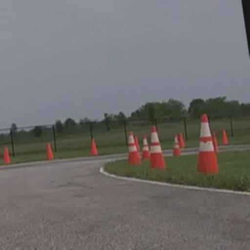
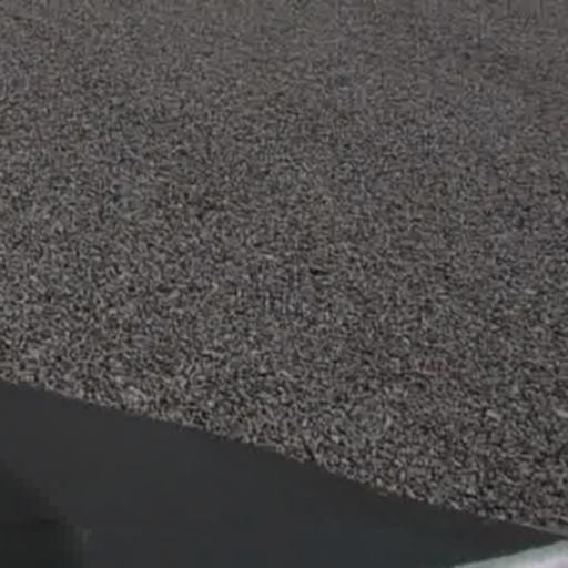
What the kart sees at it drives looks something like this:
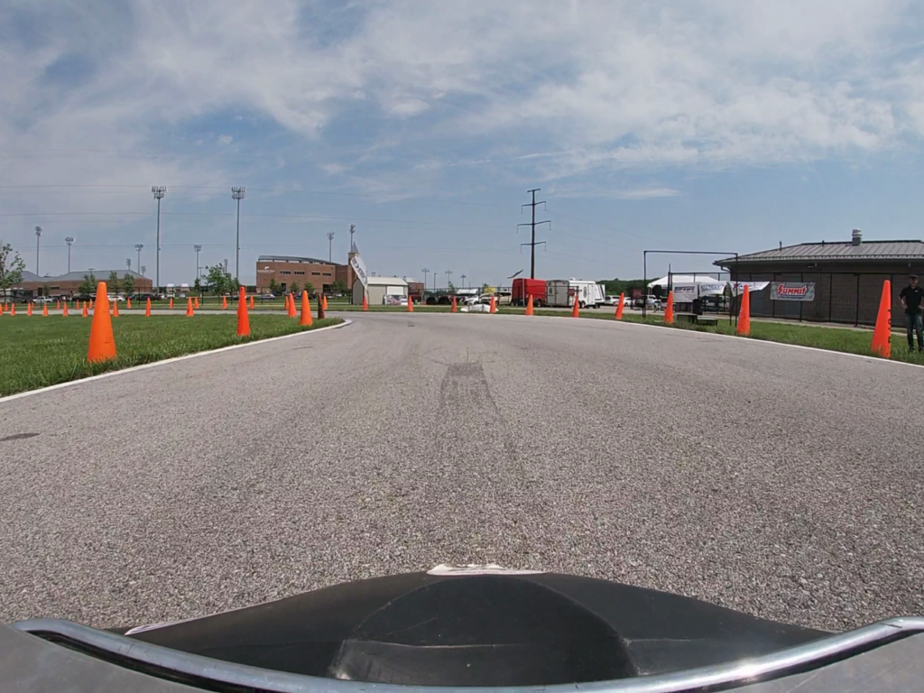
In the last season’s competition, our team acquired a Velodyne VLP-16 LIDAR (a 360° distance sensor). The kart used the height of the cones to distinguish cones marking edges of the racetrack from the ground plane. This technique left much to be desired in terms of accuracy and efficiency. Additionally, it required an expensive LIDAR sensor which increases the barrier to entry for student teams.
This season, our team began to investigate whether we could accomplish the same task using just a camera. We named this project “Coneslayer”.
Machine “Learning”
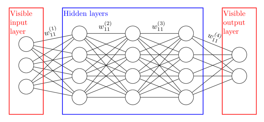
“machine learning” is a word that’s thrown around a lot in the business world. There are many flavors of this technique, but the simplest explanation of it is you tell a computer:
Given a set of inputs A and their corresponding outputs in B: Figure out a function that gets you from A → B.
The neat part about this technique is that the computer will figure out, or “learn” on its own how to get the desired output from a given input. This is used commonly in technologies today such as voice recognition, language translation, and advertising.
Data, Data, Data
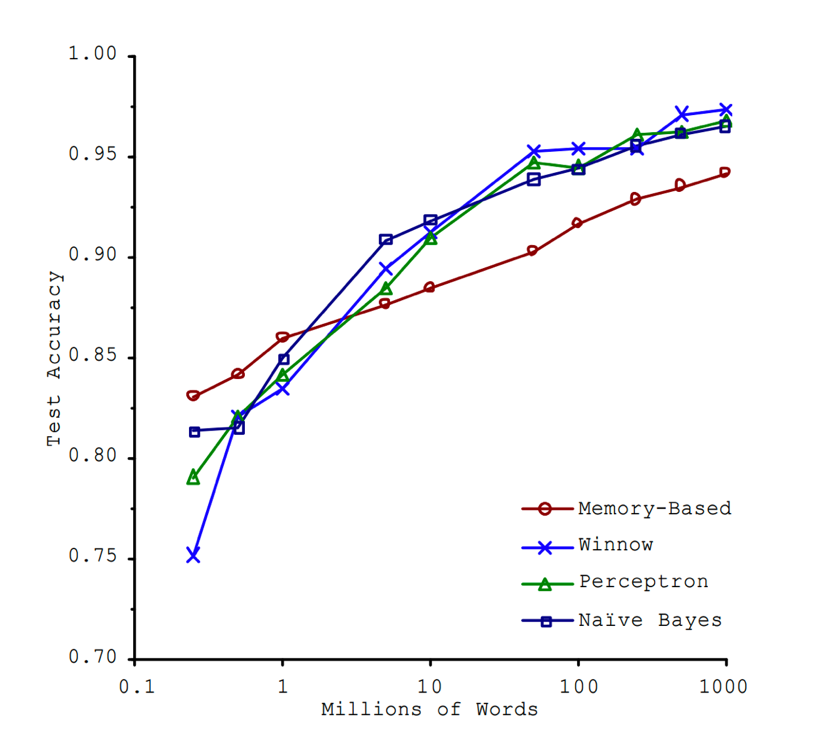
A downside of the technique however is that to accomplish this learning, a computer will need many thousands, or ideally millions, of datapoints to train itself on. In fact, the size and quality of your dataset is often more important than the ML technique itself, as two researches from Microsoft showed in 2001 in an experiment on machine translation (dubbed after as “The Unreasonable Effectiveness of Data”):
The biggest challenge our team faced in developing an object detection model for traffic cones was acquiring such a high quantity of diverse training images. To start obtaining data, I found a script which uses the wonderful ffmpeg tool to extract every high quality I-frame from a given video. I used it on 48 minutes of footage from a GoPro video camera mounted on the front of our kart as it raced around the track:
ffmpeg -skip_frame nokey -i input_vid.MP4 -vsync 0 -frame_pts true %d.jpgThis yielded about 7500 images.
I then wrote a Python script which randomly shuffled these images, then used the torchvision library to apply a random tilt, 512×512 crop, horizontal flip, color jitter, and Gaussian blur to each image: gitlab.com/KSU_EVT/autonomous-software/obtain_training_images/-/blob/master/obtain_training_images.py
This resulted in the same number of images, but now they looked something like this:

Labeling
The next task for developing Coneslayer would be to hand-label every traffic cone in each of these images 😵💫
Now you may be thinking: “Couldn’t you automate that?!?!”. The answer is: No! Not really!
Machine learning needs high quality inputs and outputs to work its magic, A → B, A → B, A → B … . If we had an algorithm generate data labels, either by color or edge detection, it’d have too many small errors for the data to be usable. Besides, if it was possible to automate this accurately, we wouldn’t be doing ML in the first place!
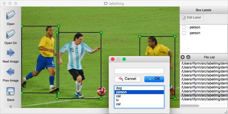
The only way to get what we’d need would be for us humans to label traffic cones by hand, clicking and dragging a bounding box over each traffic cone in each image. In our case, we chose to use a free Python program called labelImg, and the yolo .txt label format for simplicity.
Coneslayer labeling contest
We set up a shared Ubuntu laptop in our lab with this software, and started a months-long contest for image labeling. Data labeling is the most unglamorous and unrecognized part of the machine learning process. Despite its importance and impact on the resultant model, the process of labeling data by hand is slow, monotonous work. To drum up enthusiasm for the project, I staked a $25 Costco gift card as a prize to whomever labeled the most images. This coveted prize had the added benefit of permitting the winner entrance to Costco (where a hotdog + soda combo has been $1.50 since 1984).
Engagement immediately went up, and we had our results after a month of the contest:
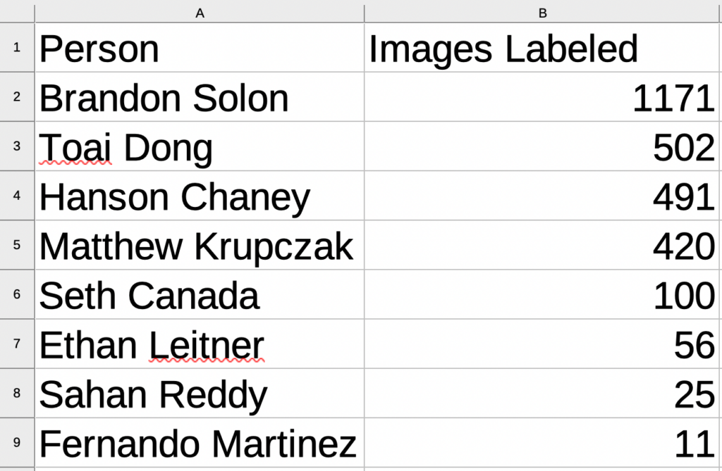
We labeled 2574 of the about 7500 images available.
Next, a colleague of mine named Ethan Leitner used a framework called You Only Look Once version 4 (YOLOv4) and a small public dataset to build a proof of concept. It was a good start, but that particular framework ran too slowly on our desired hardware and detections were not robust with such limited training data. He helped me transition to new a framework called You Only Look Once version 7 (YOLOv7), based on PyTorch, to start training on our custom data.
More data
Our results were quite poor initially, so we looked for more labeled data available for free online. We found the Formula Student Objects in Context (FSOCO) dataset from a collaboration of university teams of a different competition in Europe. Two members of our team, Sahan Reddy and Yonnas Alemu, wrote a bash script which would extract only the images and labels that contained the tag “orange_cone” or “large_orange_cone”. I wrote a Python script which converted the label files from the Supervisely to the yolo .txt format.
We couldn’t use this dataset by itself because it contained traffic cones of differing color, pattern, and sizes to those we were targeting. Ethan wrote another script which would merge our custom dataset with the FSOCO subset at a specified ratio. We mixed 3 images from the FSOCO dataset for every 1 of our own, getting us to a total of just over 10,000 labeled images for training.
Training:
One of the greatest challenges with machine learning is the sheer processing power required. To adjust the weights of a given neural net architecture, a process called “training” requires backprogation of values from millions and millions of outputs and inputs. This is a workload that is embarassingly parallel, so it makes much more sense to perform it in parallel on GPUs (in our case with over 5,000 processor cores per card) than normal CPUs. NVIDIA GPUs are superb for this task, and the latest models even feature a special hardware accelerator for common ML matrix multiplication called a tensor core. In the professional market these include the A100, V100, and H100 variants, but any consumer graphics card starting with “RTX” works fine too.
Our faculty sponsor at Kennesaw State University, Dr. Lance Crimm, provided our team access to KSU’s High Performance Computer (HPC), which was invaluable for iterating quickly in this part of the process. We could use up to 4x V100S 32Gb GPUs per node, with four nodes available should we have desired it. I got the best results however running training with just two GPUs at a time. I documented more about this process here on our team’s GitLab page if you’re interested in more technical detail.
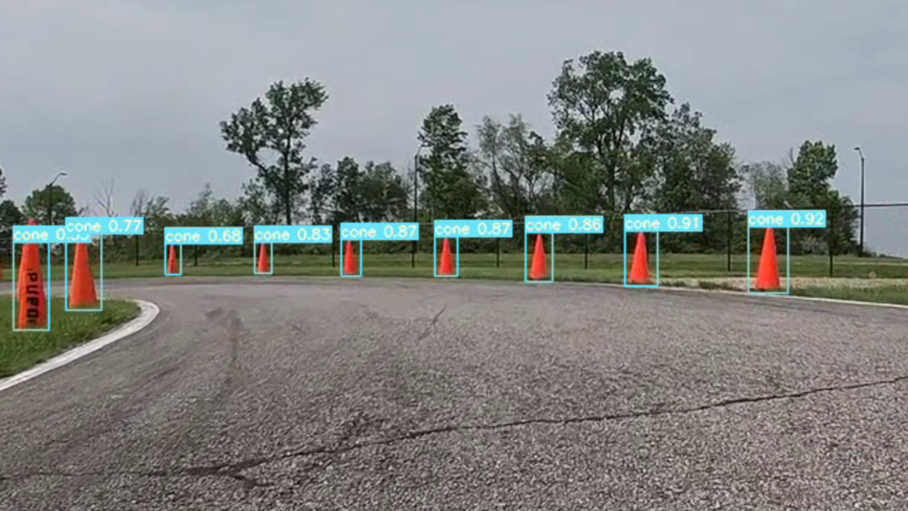
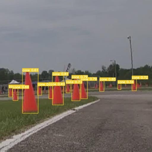
Results:
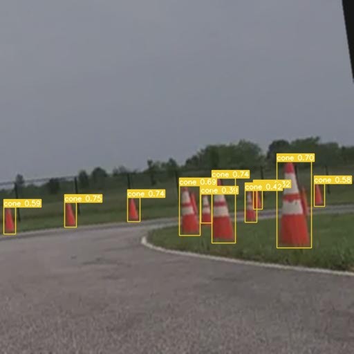

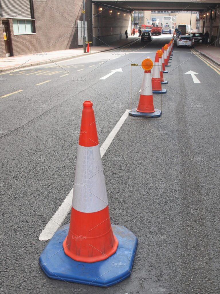
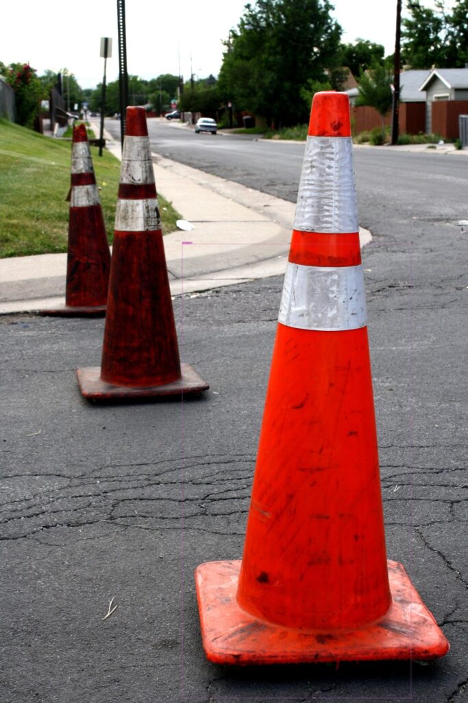
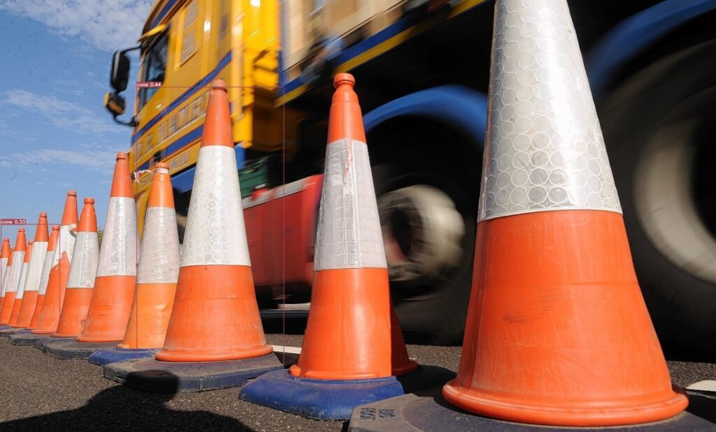
With the expanded dataset, results from Coneslayer were immediately much much better. The above images are from coneslayer-alpha-1, which was trained for two rounds of 150 epochs, with the evaluation set rotated between rounds (this technique allows for better coverage of a small dataset, without over-fitting).
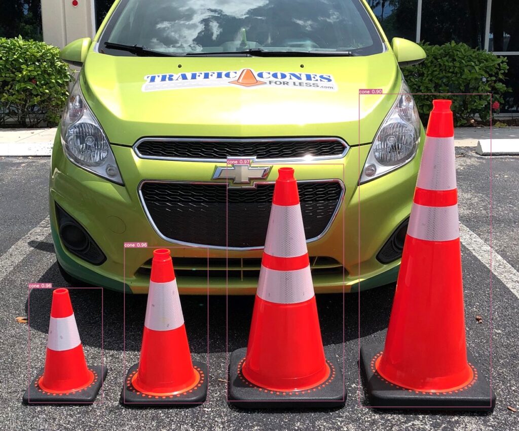
While the model worked great on traffic cones of the same size, shape, and color as the training set, it generalized poorly to real world environments:
What is a traffic cone anyways?
The challenge for our competition team is that we can’t guarantee exactly what model cone would be used for competition. Therefore we needed to make Coneslayer more generalizable.
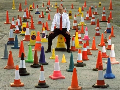
This is also where the question “what is a traffic cone?” becomes much more philosophical. Over the entire world, there are an immeasurable number of manufacturing companies and specific models of cone. To scratch the surface, one British man named “David Morgan” has the world record for his collection over 500 unique models (this also landed him on Dull Men’s Club calendar, but I digress)
The issue we encountered here is not dissimilar to that covered by Tim Anglade. He created the free hotdog / nothotdog mobile app as a promotion for the HBO TV show Silicon Valley. Something he noted after the app’s release is that his training set was mostly American hotdogs, so French users were dismayed to find their dogs weren’t recognized by the app. This kind of issue is common for the field of AI in general, and its mitigation requires significant international data sharing and cooperation.
The best we could do for Coneslayer was to do an image search for “orange traffic cone” translated into multiple languages and use the images we found in our training set. We hoped that retraining on a more diverse dataset would force the model to become more generalizable.
Cone / No Cone
To make Coneslayer more generalizable, we started a process known and “transfer learning” by retraining on a more diverse dataset of cones from around the world. The idea here is that Coneslayer already had a good understanding of how to detect an object and recognize that it is a cone, so it could learn other types of cones more easily with much fewer examples.
After training, we quickly found however that our model had generalized too far, with some pretty amusing results:
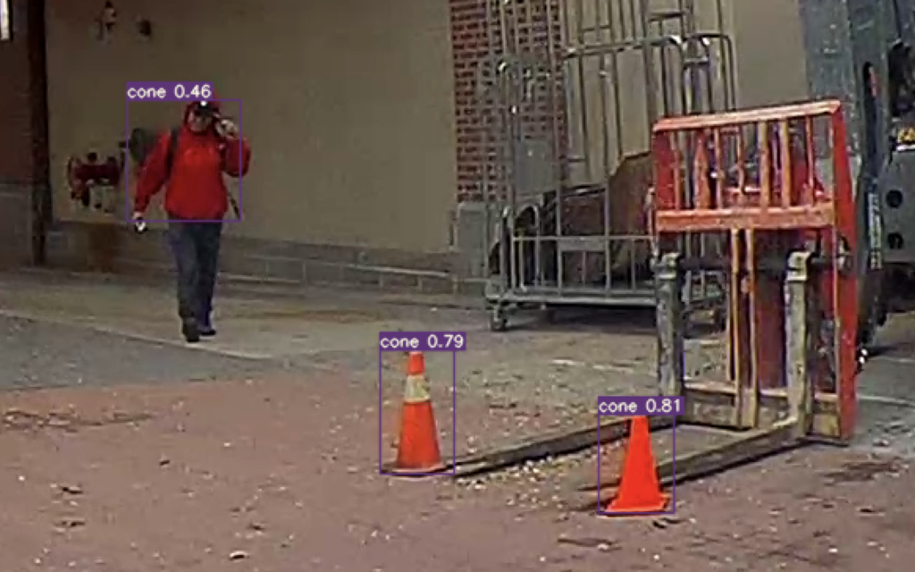
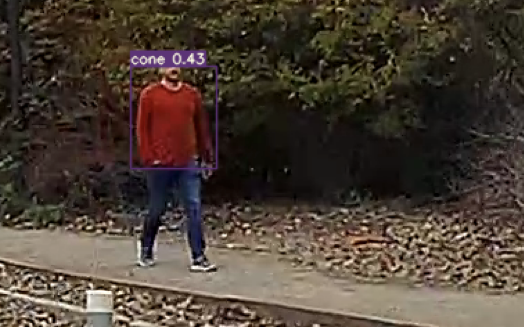
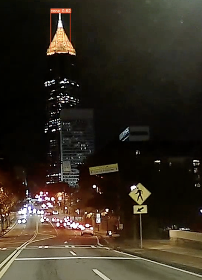
Why so many false positives?
This was another significant challenge to building Coneslayer. My hope had been that the background of most scenes in the dataset (space that didn’t contain cones) would serve as sufficient negative training data. For the level of specificity that we desired, this turned out not to be the case, and this version had much too many false positives.
The technical reason for this was that the YOLO framework discounts negative data so it doesn’t overwhelm and drown out positive information. In YOLO, this is represented as the constant λ_noobj, which is fixed at 0.5. While my preference would have been to just adjust this value, there seemed to be no option to configure it.
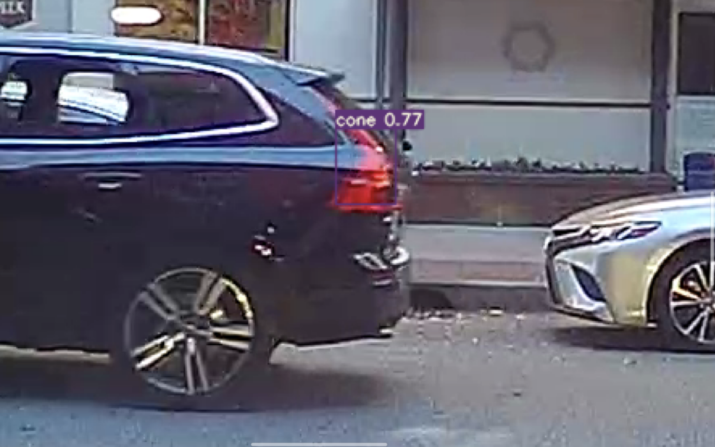
More (negative) data:
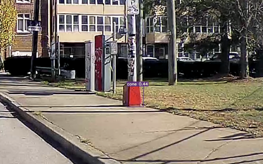
I reasoned that the only solution would be to add more negative training data to the diverse dataset for retraining. I took my most recent model (coneslayer-omega-1-robust-2), and used YOLOv7 with some bash-fu involving grep, ffmpeg, and a small Java program on about 4 hours of car dashcam video. This extracted the raw frames from the video where the model had detected what it thought was a cone. I manually searched through these images, and found about 300 where it was clear that there was not a cone in the frame (mostly the brakelights of other cars, but a few amusing examples including those above). I then created an empty .txt label file for each of these negative training images, and added them to the dataset. This fixed all the above false positive examples, save for the telephone pole with the red base.
Reflections on Coneslayer
All this above brings us to the present state of Coneslayer, as I’ve released it on GitHub.
It’s also available on the official “model zoo” of Luxonis (The company that makes our main camera):
zoo.luxonis.com
Takeaways
My first takeaway from this project is the lack of quality, open source, and well-documented frameworks for this type of project, especially including tools for data and label management. Many of the scripts we wrote to obtain, sort, shuffle, distort, segment, and conjoin datasets were very labor-intensive to create.
The documentation for the YOLOv7 framework is pretty sparse, and certain features (such as running inference on video) do not work at all if a user follows the default installation instructions. For running on the KSU HPC, I was lucky enough to get an alternative installation working using Python virtualenv’s. This is not a nag on the authors of this framework, just an example to show that the tools and processes around this type of project are not yet mature.
Methodology
As far as my own methods, there are a couple of things I would have done differently if starting this project from scratch. I would not have applied distortions to the initial homogeneous training set images because current frameworks like YOLOv7 can already take care of this with their image pre-processor. I also wish I had added many more negative examples to the heterogeneous training set to reduce the final model’s false positive rate, but this is out of scope for the needs of our student competition team.
Besides, Coneslayer is a very small model, with only about 6 million parameters. Being so small, its ability to understand complex scenes will necessarily be quite limited. This is a tradeoff we consciously made in favor of performance on small processors, such as that included on the Luxonis OAK-D Pro camera. I hope to publish the homogeneous and heterogeneous datasets soon, as well as an alternative version of Coneslayer with a larger model size.
Summary
This got quite technical here at the end, but I hope showing some of this process provides an accessible entrypoint into understanding machine learning. Science fiction writer Arthur C. Clarke says that “Any sufficiently advanced technology is indistinguishable from magic“, and this is no more the case than with machine learning. There’s a lot of snake oil out there, the hard truth though is that machine learning essentially just deals in probabilities and is never quite as perfect as you may have been led to believe. In most applications, there is neither the sufficient quantity and quality of data, nor the need for this kind of technique when an algorithmic approach can work just as well.
Matthew Krupczak is a Computer Science undergraduate at Kennesaw State University, volunteering for the KSU Electric Vehicle racing Team. His personal GitHub, featuring Coneslayer and other works, is available here. The Electric Vehicle Team’s website is ksuevt.org and its GitLab, including many public repositories such as those used in the process described above, are available at GitLab.com/KSU_EVT
Subscribe to be notified of new posts:
[mc4wp_form id=”1762″]